1.2 Representations of Motion: A Comprehensive Guide for AP Physics 1

Mastering representations of motion is key for success in AP Physics 1. These representations—ranging from graphs to equations and diagrams—offer diverse methods to describe and predict the movement of objects. This guide will help you understand these concepts thoroughly, making it easier to analyze and solve motion-related problems.

Key Representations of Motion

1. Graphical Representations 📈

Graphs provide visual insights into how objects move:

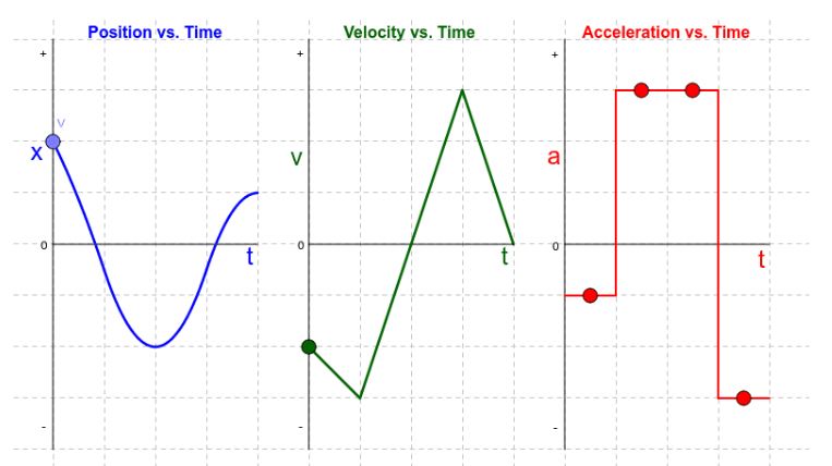
• Position-Time Graphs: Show how position changes over time.

  • Slope: Represents velocity.
  • Straight Line: Constant velocity.
  • Curved Line: Changing velocity (acceleration).

• Velocity-Time Graphs: Show how velocity changes over time.

  • Slope: Represents acceleration.
  • Area under the Curve: Represents displacement.
  • Zero Slope: Constant velocity.

• Acceleration-Time Graphs: Show how acceleration changes over time.

  • Area under the Curve: Represents change in velocity.

Example:
To find velocity from a position-time graph, calculate the slope (rise/run). To find displacement from a velocity-time graph, find the area under the curve.

2. Numerical Representations 📊

Tables and lists of numerical data can represent an object’s motion, including its position, velocity, and acceleration at different time intervals. This allows for detailed analysis and helps in identifying patterns and trends.

3. Analytical Representations 📐

Kinematic equations describe motion mathematically, allowing precise calculations of an object’s position, velocity, and acceleration over time:

• Key Equations:
  • $v = v_0 + at$
  • $x = v_0t + \frac{1}{2}at^2$
    
  • $v^2 = v_0^2 + 2ax$
    
• Variable Interpretation:
  • $x$: Displacement (m).
  • $v$: Final velocity (m/s).
  • $v_0$: Initial velocity (m/s).
  • $a$: Acceleration (m/s$^2$).
  • $t$: Time (s).

Example Problem:
A car moving at 20 m/s slows at $-3 \, \text{m/s}^2$. How far does it travel before stopping?

• Given: $v_0 = 20 \, \text{m/s}$, $v = 0 \, \text{m/s}$, $a = -3 \, \text{m/s}^2$.
• Use: $v^2 = v_0^2 + 2ax$. $$0 = 20^2 + 2(-3)x \implies x = \frac{400}{6} = 66.7 \, \text{m}$$
  

4. Diagrammatic Representations 🖼️

Sketches and diagrams illustrate an object’s motion, showing key details like displacement, velocity, and acceleration vectors. These visuals are useful for gaining an intuitive understanding of how motion unfolds over time.

Center of Mass and Motion

Key Concept: The center of mass of an object or system represents its average position of mass distribution. Applying force at this point causes linear acceleration without rotational effects.

• Equation: Acceleration of center of mass $(a)$ is related to net force $(F)$ by $a = \frac{F}{m}$.
• Practical Example: Pushing a box at its center of mass causes it to slide, while pushing at an edge may cause rotation.

Linearization of Graphs 📏

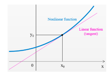
In physics, many relationships are nonlinear. Linearization converts curved data into a straight line by transforming variables (e.g., squaring the x-axis). This simplifies analysis and predictions.

Example:
To approximate the time it takes for a ball dropped from 10 meters to hit the ground:

• Nonlinear equation: $y = 10 – 4.9t^2$.
• Linearize around a specific point (e.g., $t = 1 \, \text{s}$) to create a tangent line for easier predictions.

Free Fall and Projectile Motion ☄️

Free Fall

Objects under the influence of gravity alone exhibit free fall motion:

• Acceleration due to Gravity (g): $9.8 \, \text{m/s}^2$ (rounded to $10 \, \text{m/s}^2$ for AP Physics).
• Equations:
  • $v_f = v_0 + gt$
    
  • $y = v_0t + \frac{1}{2}gt^2$
    
  • $v_f^2 = v_0^2 + 2gy$
    

Example:
A ball dropped from rest falls for $3 \, \text{s}$.

• Displacement: $y = \frac{1}{2}gt^2$. $$y = \frac{1}{2} \times 10 \times 3^2 = 45 \, \text{m}$$
  

Projectile Motion

Projectiles move in two dimensions: horizontal and vertical. Horizontal motion remains uniform, while vertical motion is influenced by gravity.

• Key Equations:
  • Horizontal: $x = v_xt$
    
  • Vertical: $y = v_{0y}t + \frac{1}{2}gt^2$
    
• Breaking Motion into Components: Use trigonometric functions to resolve initial velocity into horizontal and vertical components.

Example:
A cannonball launched at $30^\circ$ with an initial speed of $20 \, \text{m/s}$.

• Time of Flight: $$t = \frac{2v_{0y}}{g} \implies v_{0y} = v_0 \sin(30^\circ) = 10 \, \text{m/s} \implies t = \frac{2 \times 10}{10} = 2 \, \text{s}$$
  
• Range: $$x = v_{0x}t \implies v_{0x} = v_0 \cos(30^\circ) \approx 17.3 \, \text{m/s} \implies x = 17.3 \times 2 = 34.6 \, \text{m}$$