AP Physics C: Mechanics Score Calculator
2027 practice index, out of 100. Enter current-format practice scores to see a weighted practice index. This is not an official composite or an AP 1–5 score prediction.
Use a complete 42-question multiple-choice section and the four free-response task scores below. Enter all five whole-number scores. Blank is missing; 0 is an entered score. Sources and study guide
An AP Physics C: Mechanics score calculator is most useful when it helps you decide what to practice next. A total alone cannot reveal whether you misunderstood a force, lost a sign during integration, or left a graph unexplained. This guide connects a transparent practice index with the reasoning that earns stronger mechanics responses: choosing a system, building a representation, applying a physical law, and checking what the mathematics means.
The guide is written for the 2027 exam and uses the announced May 2027 format. Its worked problems are original learning exercises, not reproduced exam questions. Use them with your class materials and the scoring guide that belongs to each released question. For other subjects, visit the AP score calculator collection; for broader preparation, browse the study guides.
How to use the AP Physics C: Mechanics score calculator
Enter the number of multiple-choice answers you got correct and the points earned on each free-response question. For this practice model, the input limits are forty-two multiple-choice answers and four free-response maxima of ten, twelve, ten, and eight points. Those free-response limits appear in the current official course overview and recent scoring materials. Check the rubric before transferring results from an older practice set; a question with a different maximum does not fit an input merely because its topic looks familiar.
The calculator assigns half of its practice index to each section. It divides your multiple-choice count by forty-two and your combined free-response points by forty, then applies the two fifty-point weights. Pooling the free-response points is an editorial practice-model choice. It does not claim that College Board uses this exact raw-point transformation when setting an exam’s official composite. The output is a weighted practice index out of one hundred, with two decimal places for convenient comparison.
Practice index = 50(MC ÷ 42) + 50[(MR + TBR + EDA + QQT) ÷ 40]
Keep that distinction in mind when using the examples below. The first student profile has twenty-eight correct multiple-choice answers and twenty-four combined free-response points. Improving four multiple-choice answers increases the index by about 4.76 points. Improving one raw point on each free-response question increases it by exactly five points. This comparison describes the calculator’s arithmetic, not the relative difficulty of earning those gains or a guarantee about the eventual AP score.
| Profile | MC / 42 | MR / 10 | TBR / 12 | EDA / 10 | QQT / 8 | Index / 100 |
|---|---|---|---|---|---|---|
| Starting profile | 28 | 6 | 7 | 6 | 5 | 63.33 |
| Four more MC answers | 32 | 6 | 7 | 6 | 5 | 68.10 |
| One more point per FRQ | 28 | 7 | 8 | 7 | 6 | 68.33 |
Do not convert these indices into an invented table of AP scores from one to five. Official score setting involves exam-specific evidence, and a practice collection may differ in content, difficulty, timing, and scoring reliability. A better comparison uses similarly demanding sets completed under similar conditions. Record the index alongside a short error log and your confidence in the marking. If a teacher changes an ambiguous rubric decision, revise the input rather than treating the earlier decimal as a precise measurement of ability.
Prepare for the current 2027 exam format
The announced 2027 exam has forty-two multiple-choice questions in eighty-five minutes and four free-response questions in ninety-five minutes. Each section contributes fifty percent of the exam score. Together, the working sections total 180 minutes. These details replace the earlier forty-question, eighty-minute multiple-choice section and one-hundred-minute free-response section. The older thirty-five-question multiple-choice and three-question free-response format is also unsuitable for a 2027 full-length simulation. Check a resource’s date before using its pacing advice.
| Section | Questions | Time | Published weight |
|---|---|---|---|
| Multiple choice | 42 | 85 minutes | 50% |
| Free response | 4 | 95 minutes | 50% |
The standard administration is hybrid digital: students complete multiple choice and view free-response prompts in Bluebook, then handwrite free-response answers in paper booklets. Practice switching attention between a displayed question and a written solution. Put labels and explanations directly beside the relevant mathematics so that a reader can follow the work without reconstructing your intentions. Calculator use is permitted, but familiarity with a permitted device and the provided reference material matters more than memorizing button sequences. Bluebook AP test previews are untimed and unscored; use them for interface familiarity rather than timed score comparisons.
The regular exam is listed for May 3, 2027, in Session 1. Confirm your school’s reporting instructions and the official start-time guidance rather than assuming the session label means the same local clock time everywhere. The four free-response task types are mathematical routines, translation between representations, experimental design and analysis, and qualitative/quantitative translation. Prepare all four kinds of work; knowing how to compute an answer is only part of showing that you understand a physical model.
Choose study priorities without skipping whole units
The course develops calculus-based mechanics through seven units. The table gives the published multiple-choice weighting ranges, which describe coverage rather than a promise of exact question counts on your practice test. A question can also require skills learned across several units. A rolling object’s speed, for example, may involve translation, rotational inertia, energy, and a constraint linking linear and angular motion. Learn those connections instead of treating each unit as an isolated formula collection.
| Unit | Weighting range | A useful review question |
|---|---|---|
| Kinematics | 10% to 15% | What do a graph’s slope and signed area mean? |
| Force and Translational Dynamics | 20% to 25% | Which external interactions change this object’s motion? |
| Work, Energy, and Power | 15% to 25% | Which transfers or transformations change the system’s energy? |
| Linear Momentum | 10% to 20% | Is the external impulse negligible during this interval? |
| Torque and Rotational Dynamics | 10% to 15% | About which axis should torque and inertia be evaluated? |
| Energy and Momentum of Rotating Systems | 10% to 15% | Which rotational quantity is conserved under these conditions? |
| Oscillations | 10% to 15% | What makes the restoring force proportional to displacement? |
Choose the next topic using both frequency and evidence from your own work. If you repeatedly omit a force or use velocity in place of acceleration, fixing Newton’s second law can improve several units at once. If your setup is usually correct but graphs lack scale and units, representation practice may produce a more immediate gain. Diagnose the actual bottleneck before assigning another hour of undirected reading.
Keep three short categories in an error log: physical model, mathematical execution, and communication. A wrong conservation assumption belongs in the first category; a dropped integration constant belongs in the second; an unlabeled axis belongs in the third. Some mistakes span categories, so include a one-sentence repair. That sentence should tell your future self what to do differently, such as checking external impulse before conserving momentum.
Start with a system and a readable diagram
Before manipulating symbols, identify the object or collection of objects you are analyzing. A free-body diagram for one cart contains forces exerted on that cart by other objects. A diagram for two connected carts treated as a single system excludes their mutual interaction from the external-force total. Neither choice is automatically better. Choose the boundary that makes the requested quantity accessible, then keep the boundary consistent throughout the argument.
Draw forces from a simple point or outline, label their agents or physical types, and choose positive axes. Avoid adding a separate arrow labeled net force beside the forces you plan to sum; that can double-count the resultant as though it were another interaction. Likewise, velocity is not a force. An object can move right while accelerating left, and a force diagram should represent the acceleration-producing interactions without trying to imitate the direction of travel.
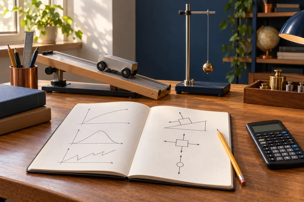
Connect the drawing to an equation for each relevant axis. For the cart shown, zero vertical acceleration implies that the normal force equals the weight because those are its only vertical forces. That equality would change if the pull had an upward component. Horizontally, a larger applied force than kinetic friction produces rightward acceleration. State these conditions; writing the familiar equality without checking the actual force directions is a common source of hidden errors.
Connect derivatives and integrals to motion
Calculus gives a language for changing motion. Velocity is the time derivative of position, and acceleration is the time derivative of velocity. Definite integrals run the reasoning in the other direction: the signed area under an acceleration graph gives a change in velocity, while the signed area under a velocity graph gives displacement. Initial conditions supply the missing starting value. A correct antiderivative without the correct initial condition can describe a different motion.
vx = dx/dt; ax = dvx/dt; Δx = ∫t1t2 vx dt
Consider an original one-dimensional model with position given by x(t) = 2 + 4t − t2, where position is in meters, time is in seconds, and the coefficients carry the corresponding units. Differentiation gives velocity 4 − 2t in meters per second and constant acceleration of negative two meters per second squared. The object initially moves in the positive direction, stops momentarily at two seconds, and then moves in the negative direction. Zero instantaneous velocity does not imply zero acceleration.
At zero, two, and four seconds, the positions are two, six, and two meters. Over the full interval the displacement is zero, but the distance traveled is eight meters. The positive and negative areas on the velocity graph cancel for displacement; they add in magnitude for distance. This is a useful test of whether you are integrating velocity or speed. On the position graph, the turning point has zero slope and downward curvature, consistent with the velocity and acceleration calculations.
For a variable acceleration, resist using constant-acceleration formulas automatically. Suppose a two-kilogram cart starts at rest and experiences a net horizontal force F(t) = (6 N/s)t for two seconds. Its acceleration grows linearly, so integrating gives a final speed of six meters per second and a displacement of four meters. Using the final acceleration for the entire interval would overestimate both. Check the force units, integrate over the stated interval, and explain why your result matches the increasing slope of the velocity graph.
Use Newton’s laws with constraints and limiting cases
Newton’s second law relates the vector sum of external forces to the acceleration of the selected object or system. It does not say that every force equals mass times acceleration. When several objects share a string, first write a separate equation for each object with a consistent acceleration constraint. Decide whether the string is idealized as massless and inextensible and whether the pulley has negligible rotational inertia. Those assumptions determine whether equal tensions are justified.
In an original example, a three-kilogram cart on a frictionless horizontal track connects over an ideal pulley to a hanging two-kilogram mass. Take the cart’s motion toward the pulley and the hanging mass’s downward motion as positive. The cart equation is T = Ma, while the hanging mass equation is mg − T = ma. Adding them cancels the internal tension and gives acceleration mg/(M + m). With gravitational acceleration 9.8 meters per second squared, the acceleration is 3.92 meters per second squared and the tension is 11.76 newtons.
The tension is smaller than the hanging weight because that mass accelerates downward. Check two limiting cases before moving on: as the hanging mass approaches zero, the acceleration approaches zero; as the cart mass approaches zero, the acceleration approaches gravitational acceleration in this ideal model. A result exceeding gravitational acceleration here would signal an error in the equations or signs. These checks are useful even when the question requests only a symbolic expression.
For circular motion, identify the real forces that have components toward the center. The radial acceleration has magnitude v2/r, but there is no extra interaction called centripetal force to add to the diagram. A satellite’s gravitational force can supply its radial acceleration. Setting the inverse-square gravitational force equal to the required radial resultant gives orbital speed proportional to the inverse square root of orbital radius for a circular orbit around a fixed central mass. Increasing radius therefore lowers that speed.
Choose energy when forces vary with position
Energy methods are often efficient when the question asks for a speed after motion through a distance. Begin by identifying the system and which interactions are represented by potential energy. If the Earth and object are inside the system, gravitational potential energy can describe their interaction. If a spring is included, elastic potential energy can be included as well. Work done across the boundary and changes in internal energy must still be accounted for when relevant.
A half-kilogram block released from a spring compressed by 0.10 meters illustrates the bookkeeping. For an ideal spring with stiffness 200 newtons per meter on a frictionless horizontal surface, the initial elastic energy is one joule. When the spring reaches its natural length, that energy has become the block’s kinetic energy, giving a speed of two meters per second. Doubling the compression would quadruple the initial energy and double the resulting speed, provided the same assumptions remain valid.
For a varying force, calculate work using the area under the force-position curve. Suppose a net force follows Fx = (6 N/m)x − (2 N/m2)x2 from one to three meters. Integration gives work of twenty-thirds of a joule, approximately 6.67 joules. A two-kilogram object starting at rest therefore reaches approximately 2.58 meters per second. The force is nonnegative throughout the interval and positive before the final endpoint, so positive work and increased kinetic energy are physically consistent.
Wnet = ∫ Fx dx = ΔK; Fx = −dU/dx; P = F · v
A potential-energy graph offers another representation of the same interaction. Force points toward decreasing potential energy, and a stable equilibrium occurs at a local minimum because small displacements produce restoring forces. Power describes the rate of energy transfer, not the amount stored. For a force parallel to velocity, instantaneous power is force times speed; when the vectors are perpendicular, that force does no instantaneous work even though it can change the direction of motion.
Separate momentum conservation from energy conservation
Momentum is especially useful for short interactions such as collisions. Define the collision system, choose a signed axis, and evaluate the external impulse over the collision interval. Internal forces can be large while canceling in the system’s total momentum change. Negligible external impulse allows total momentum to remain approximately constant. It does not imply that each object keeps its own momentum, or that the total kinetic energy stays constant.
For an original collision, a 0.40-kilogram cart moving right at three meters per second sticks to a 0.60-kilogram cart moving left at one meter per second. With right positive, the initial total momentum is 0.60 kilogram meters per second. The combined one-kilogram mass therefore moves right at 0.60 meters per second if external impulse is negligible. Adding the incoming speed magnitudes would incorrectly erase the opposing directions.
The initial kinetic energy is 2.10 joules, while the final kinetic energy is 0.18 joule. The decrease of 1.92 joules is consistent with a perfectly inelastic collision: energy changes into other forms, including deformation and thermal energy. Total energy remains conserved for a sufficiently inclusive system, but mechanical kinetic energy is not. State which conservation statement you are using and why its conditions apply.
Impulse also connects force graphs to momentum. A triangular force-time pulse with a base of 0.20 second and a height of twelve newtons delivers an impulse of 1.20 newton seconds if its force remains in one direction. Applied to a 0.30-kilogram object, that impulse changes velocity by four meters per second. The graph’s shape matters: multiplying the peak force by the full duration would double the actual impulse in this example.
Track the axis in rotational mechanics
Rotational problems require an axis as well as a system. Torque depends on the perpendicular distance from that axis to the force’s line of action, and rotational inertia depends on how mass is distributed about the same axis. A larger total mass does not automatically imply a larger rotational inertia if the distribution and axis differ. Write the axis beside the diagram before selecting an inertia expression or applying the parallel-axis theorem.
For a uniform disk of mass two kilograms and radius 0.30 meter, the rotational inertia about its central symmetry axis is 0.090 kilogram meters squared. A tangential four-newton force at the rim produces torque of 1.20 newton meters and angular acceleration of approximately 13.3 radians per second squared, assuming no other torque about that axis. A radial force of the same magnitude would produce zero torque about the center because its line of action passes through the axis.
Rolling without slipping combines translation and rotation. For a solid sphere released from rest through a vertical drop h, energy conservation and the condition v = ωR give v2 = 10gh/7. For a one-meter drop with gravitational acceleration 9.8 meters per second squared, the final speed is approximately 3.74 meters per second. A pointlike object sliding without friction through the same drop would reach approximately 4.43 meters per second because none of its kinetic energy would be rotational.
The rolling model requires enough static friction to prevent slipping. Static friction can exert a torque even when, in the ideal rigid-body model on a stationary surface, it transfers no energy at the instantaneous contact point. If slipping occurs, the rolling constraint cannot simply be retained. Explain the assumed contact behavior before substituting angular speed for linear speed.
Angular momentum provides a separate tool. If a rotating system experiences negligible external torque about a chosen fixed axis, its angular momentum about that axis remains constant. Bringing mass closer to the axis reduces rotational inertia and increases angular speed. The rotational kinetic energy can increase because internal work is done during the rearrangement. Conservation of angular momentum therefore does not license a second, automatic assumption that rotational kinetic energy is unchanged.
Recognize the restoring relationship in oscillations
Simple harmonic motion follows when the restoring force is proportional to displacement from equilibrium and opposite in direction. For an ideal horizontal mass-spring oscillator, Newton’s law gives acceleration equal to negative stiffness divided by mass, multiplied by displacement. The negative sign describes restoration toward equilibrium. It does not mean velocity is always negative, and it does not mean the object is always slowing down.
Take a half-kilogram mass attached to a spring with stiffness 200 newtons per meter and oscillation amplitude 0.10 meter. The angular frequency is twenty radians per second, the period is approximately 0.314 second, and the maximum speed is two meters per second. At a displacement of positive 0.060 meter, acceleration is negative twenty-four meters per second squared. Energy gives a speed magnitude of 1.60 meters per second there, but the sign of velocity depends on whether the mass is moving toward or away from the positive turning point.
Use this example to connect phase and energy. At either turning point the speed is zero and the acceleration magnitude is greatest. At equilibrium the speed magnitude is greatest and acceleration is zero. A position graph and an acceleration graph are opposite in sign at each instant; the velocity graph is shifted relative to position. These relationships let you reject an inconsistent sketch without calculating every point.
For a simple pendulum, the familiar period expression assumes small angular displacements and an idealized point mass on a light support. Its leading-order period is proportional to the square root of length and independent of bob mass. Doubling length therefore multiplies the period by the square root of two. State the small-angle condition rather than extending the formula to arbitrarily large swings.
Design experiments that test a relationship
An experimental plan should make the desired quantity measurable. Identify the independent variable, the dependent variable, the controls, and the equipment needed to collect them. Explain the procedure with enough detail that another student could repeat it. Saying to take measurements and draw a graph leaves the important decisions unstated: what gets varied, what gets recorded, and how the slope or intercept answers the question.
To estimate a spring’s stiffness dynamically, measure the oscillation period for several known attached masses while keeping amplitudes small and the same spring in use. Time multiple complete cycles for each trial and divide by the number of cycles. Repeat trials at each mass, then graph period squared vertically against mass horizontally. For an ideal massless spring, the slope is four times pi squared divided by stiffness. A measured slope of 0.200 seconds squared per kilogram would imply stiffness of approximately 197 newtons per meter.
T2 = (4π2/k)m; k = 4π2/(slope of T2 versus m)
That linearization makes the slope’s meaning explicit. Reversing the graph axes changes the slope and the extraction formula. Check units before reporting stiffness: dividing a dimensionless factor by seconds squared per kilogram yields kilograms per second squared, equivalent to newtons per meter. An unexpected nonzero intercept may indicate an omitted contribution, such as effective oscillating spring mass or an unaccounted mass holder, rather than merely random measurement noise.
Distinguish random scatter from systematic shifts. Timing several cycles reduces the fractional effect of a similar absolute start-stop uncertainty, while averaging repeated trials helps characterize variation. Neither step repairs a consistently miscalibrated clock. If a measured period is systematically two percent too large, its square is approximately four percent too large for a small relative error, and the inferred stiffness from the slope is approximately four percent too small. Explain the direction of the effect through the relationship, not just the phrase human error.
When comparing a model with data, inspect the pattern of residuals and the size of plausible measurement uncertainty. A smooth curve in residuals can indicate that the linear model omits a dependence. Do not force a best-fit line through the origin solely because the ideal equation predicts zero intercept; first consider whether the experiment measures additional masses or offsets. A useful conclusion states whether the observations support the model within the experiment’s limitations and names a specific improvement that addresses a documented weakness.
Write free responses that expose your reasoning
For mathematical routines, begin with a relevant law and derive the requested relationship symbolically before inserting numbers when the prompt calls for a derivation. Define any additional variables, preserve vector directions or signed components, and show the substitution that connects one step to the next. A correct numerical result is less informative when the reasoning is invisible. When you are stuck, an accurate diagram and a valid governing relationship can still communicate what you understand.
For translation between representations, check that the graph, equation, and explanation describe the same system and interval. A velocity graph’s intercept should agree with the stated initial velocity; its slope should agree with acceleration. A potential-energy curve should imply forces consistent with the force diagram. Label axes with quantities and units, show meaningful intercepts and extrema, and distinguish a qualitative sketch from a graph that requires numerical scale.
For qualitative/quantitative translation, make a prediction, derive or inspect a relationship, and explain why the result supports or changes the prediction. For example, if the hanging mass in the earlier cart system increases while the cart mass stays fixed, the acceleration increases but remains below gravitational acceleration. The expression mg/(M + m) supports both claims. Merely writing that a quantity increases because the formula says so misses the opportunity to connect the competing numerator and denominator changes.
For experimental design and analysis, keep procedure, measurement, analysis, and conclusion connected. A proposed graph must use quantities your procedure actually measures. A claimed uncertainty reduction must address an identified source of uncertainty. When reviewing a released response, compare each part with its own official scoring guide rather than awarding points for overall length, handwriting neatness, or a final answer that happens to match.
Build a repeatable study and review cycle
Begin a study cycle with a mixed set completed without looking at solutions. Record elapsed time, confidence, and the reason for each error. Then choose one specific repair, such as integrating a variable force correctly or distinguishing the system’s external forces from internal ones. Review the relevant idea briefly and solve a new problem that changes the surface details while retaining the same physical structure.
Return to the repaired skill after a delay. A solution that feels obvious immediately after reading it may still be difficult to reconstruct independently the next day. Mix old and new material so that you must choose the method rather than being told which chapter’s equation to use. Include explanation-only prompts, graph sketches, dimensional checks, and experimental plans alongside numerical calculations.
As the exam approaches, practice longer sets under the current section timings and use the actual response medium. Eighty-five minutes for forty-two multiple-choice questions averages a little over two minutes per question, but individual questions vary. Ninety-five minutes for four free responses averages just under twenty-four minutes per question; it is a planning reference rather than a rule to abandon a nearly finished response. Leave time to inspect units, missing parts, and inconsistent signs.
After scoring, update the practice calculator and compare the error patterns before celebrating or worrying about the total. An index that stays similar while conceptual errors shrink and timing improves can still represent progress. The next useful goal is concrete: produce a correct force diagram without prompting, explain the sign of work, or extract a physical constant from a graph. Those changes give your next practice score a stronger foundation.
Frequently asked questions
Does this calculator predict my official AP score?
No. It reports an editorial weighted practice index using the stated inputs and section weights. It does not supply an official composite transformation or a universal conversion to an AP score from one to five. Use it to compare similar practice attempts and identify whether multiple choice, free response, or both need attention.
Can I enter results from an older exam?
Only when the question counts and scoring maxima match the model. Older materials can still provide valuable mechanics practice, but different denominators make a direct transfer misleading. Score the questions with their own rubrics and review the physics separately rather than squeezing incompatible totals into the current calculator.
How much calculus should I practice?
Practice calculus as part of physical reasoning: derivatives of motion functions, definite integrals for displacement, impulse and work, and relationships between force and potential energy. Include units and initial conditions. Understanding what a derivative or integral represents helps you choose an operation and recognize an answer that is mathematically tidy but physically wrong.
Should I memorize every equation on the reference sheet?
Focus on recognizing each equation’s meaning, variables, assumptions, and useful rearrangements. Practice finding the provided relationships quickly, then deriving the expression the question actually requires. A reference sheet cannot choose your system, decide whether momentum is conserved, or determine the sign of a force component for you.
What is the best way to improve free-response performance?
Write complete solutions before checking a rubric, then identify exactly which reasoning or representation was missing. Redo that part from a blank page and attempt a different problem using the same skill. Include all four task types in your practice so that experimental reasoning and graph creation develop alongside algebra and calculus.
Sources
Exam details checked October 5, 2026. The 2027 update takes precedence where an older course document lists earlier question counts or section timings. All instructional examples and hypothetical calculator profiles in this guide are original.
- College Board: AP Physics C: Mechanics exam overview and 2027 format
- College Board: course and exam description clarifications and 2027 corrections
- College Board: course units, weighting ranges, and science practices
- College Board: current course overview with free-response point maxima
- College Board: AP Physics C: Mechanics course and exam description
- College Board: 2026 free-response scoring guidelines
- College Board: released mechanics questions and scoring information
- College Board: Bluebook test previews and practice
- College Board: AP calculator policy
- College Board: score setting and scoring
- College Board: exam start-time guidance